

More than ever, today's database administrator is under the gun to squeeze every last drop of performance from the databases they manage. And that's not an easy task considering the complex client/server, Internet/Intranet architecture a DBA must navigate. In addition to daily headaches, one big problem DBAs face is keeping up to date with the most current product improvements. With each new release, DBMS vendors introduce performance-enhancing features in their core offerings to improve the speed and accuracy with which they deliver information. Staying current on these enhancements can be a difficult task for DBAs, who find themselves continually fighting fires, building physical data models, performing backups, and the like. Sometimes it's tempting just to upgrade to the most current software release without digging in and finding out if it contains any real, useable updates.
Take my advice: Resist this temptation. I know it's time-consuming as well as wearisome to test out and benchmark the various enhancements and new development methods that the database giants keep churning out, but at times there's gold in those hills for administrators who diligently plug away. For example, Oracle Corp. has, beginning with version 7.0, continually added new features to its database kernel that can result in dramatic performance improvements for those who take the time to understand and implement them correctly. As I worked through some of the features and methods, I literally found my eyes popping out from the different benchmarks I took. I am still amazed by what a difference you can make in a database or application by making use of a new enhancement or rewriting your SQL. As you'll see, it's getting easier to create a big difference from a small change.
However, the basic parallel feature of Oracle7, the parallel query option, has received little fanfare from the database trenches -- and this is unfortunate. Used properly, the parallel query option has the ability to turn around time-consuming tasks in a hurry.
The parallel query option works like this: In response to a user's request, Oracle is able to divide the work needed to produce the end result between a number of "query servers" that work on the request simultaneously. (See Figure 1.) At the helm of this process is the "query coordinator," which kicks off the parallel execution of the user's statement to the query servers. The query coordinator also handles and assembles the results from those servers back to the user to complete the request. Without the parallel query option, a user's demands are always performed by a single server process, which can be constraining. To help eliminate this bottleneck, Oracle has chosen to enable the parallel query option for the most common statements a user issues:
From the SQL side, the way the parallel query option is invoked depends on the operation you're performing --whether it's DDL or DML. Let's first look at SELECT statements because that's where huge amounts of time can be eaten up by either inefficiently written queries or large data volumes. To begin with, you need to understand that the primary use of the parallel query option in SELECT statements is in table scan operations. The other types of SELECT queries that will benefit include joins and sorts. This is important because it impacts the methods you use to invoke the parallel query option. You want to use it where you'll get the most bang for the buck.
I've used the parallel query option for SELECT statements primarily for setting the parallel degree of tables via DDL and for using hints in SQL statements. The first method involves setting an Oracle table's default degree of parallelism, which you can do either at object creation or afterwards using the ALTER TABLE command. Say you have a several-million-row table that is scanned many times in a heavy OLAP environment. To ensure that any table scans on the table are performed in parallel, you can use a statement such as:
ALTER TABLE BIG_TABLE PARALLEL 3
This command forces table scans to use a minimum of three query servers when processing a user's request. I use these types of statements often to benchmark scan results and see where the law of diminishing returns takes over. For many of my scenarios, three query servers give me the highest degree of performance on my dual-processor, Intel-based machines. Your story could be different, so be sure to run your own tests and find the point where adding additional query servers doesn't produce any noticeable benefit.
The second method for using the parallel query option that I make use of is SQL hints. Hints force the Oracle optimizer to take a different route than it would normally take on its own. One of the many Oracle hints you can use specifies a degree of parallelism for a table that's applied on the fly. Say you have a large table you want to perform a count on. A scan operation will be applied, so you want it performed in parallel. To execute this operation, you can use a SQL statement such as this:
SELECT /*+ FULL(BROKERDETAILS)
PARALLEL(BROKERDETAILS,3) */
COUNT(*)
FROM BROKERDETAILS;
This statement forces the optimizer to execute the aggregate SQL request using three query servers. Note the use of the FULL hint in addition to the PARALLEL hint in the SQL above. Because Oracle's parallel query option only works on table scans for SELECT statements, we need to force the optimizer to perform a full table scan on BROKERDETAILS to ensure that the parallel option will be invoked. These types of hints should be tested by developers to see if application performance can be improved by any measure. Hints can normally be specified in most of the 4GL client/server tools (such as PowerBuilder), so if the parallel query option is available to you, why not try hints to see if you can gain any performance ground?
Can the parallel query option really make a eye-opening performance difference? Let's do a quick comparison and see. (All benchmarks that follow were produced on a Compaq dual Pentium 100MHz server, 128MB of RAM running Windows NT 3.51 server, and Oracle 7.3.2.2.0 Enterprise.) For this test, we'll use the following SQL statement:
SELECT COUNT(*)
FROM BROKERHEADER A,
BROKERDETAILS B
WHERE A.TXNID = B.TXNID
The BROKERHEADER table has about 6,000 rows in it, and the BROKERDETAILS table has 1.2 million rows. The query plan used by Oracle is as follows:
SORT [AGGREGATE]
  NESTED LOOPS
    TABLE ACCESS [FULL] of
     BROKERDETAILS
    UNIQUE INDEX [UNIQUE SCAN] of
     BROKERHEADER_X(TXNID)
The larger table, BROKERDETAILS, is accessed by Oracle by a full table scan. Because this is the case, we'll apply a default degree of parallelism to it by issuing this statement:
ALTER TABLE BROKERDETAILS
PARALLEL 3;
Now the scan will be executed in parallel by three query servers. The end result for both parallel and nonparallel operations is in Table 1. The performance improvement using the parallel query option is 62 percent -- not bad for just making one small change. If you like what you see here, experiment on your own using different numbers of query servers to see if you can improve the response times for some of the bigger table scans you experience on your system.
Another way I've used the parallel query option that has proven useful is in regard to index creations for large tables. For sizable data warehouses or data marts, it's typical during batch loads or complete table refreshes for any indexes on tables to be dropped to speed data insertion (because not only is the table updated, but each index is as well). After the load has completed, the indexes are then rebuilt, and on large tables, this process can take some time. Fortunately, the parallel query option can be used to speed this process.
Let's look at an example. I need to create a nonunique index for a DATE column on a two million row table. First I'll do it in the normal fashion, and then I'll create the index using a parallel degree of 10. The results are shown in Table 2. As you can see, gains such as this can really help reduce the load times required to get a data warehouse or mart up to date.
The good news for most Oracle users is that the company no longer sells the parallel query option as an add-on feature of its enterprise product -- it now comes bundled in. Unfortunately, users of Oracle's lower-end database products (Personal Oracle, Workgroup, and so on) won't find the same benefit, at least not for now.
A bitmap index differs from a normal B-tree index in that it works best on columns with low cardinality. A B-tree index stores ROWIDs for each key that in turn points to the rows in the table containing the key value. The value of B-tree indexes can be found in situations where columns contain data with many possible values, such as CUSTOMER_NUMBER in a CUSTOMER table.
A bitmap index, on the other hand, assigns a bitmap for each key value instead. Each bit in the bitmap scheme matches a possible ROWID, and if the bit is set, it indicates a hit. That makes bitmap indexes ideal for columns that have values that are often identical.
In addition to performance benefits, bitmap indexes offer the added feature of requiring less storage space than their B-tree counterparts. When created on low-cardinality columns, the compressed bitmap index format can equal only 25 percent of a normal B-tree index, Oracle claims. The reverse, however, is true for bitmap indexes created on high-cardinality columns, so be sure of the data distribution in your targeted table column(s) before creating any bitmap indexes.
A bitmap index is created in the normal way you'd expect to create an index. A sample bitmap index creation is:
CREATE BITMAP INDEX
BROKER_DETAILS_B1 ON
BROKER_DETAILS (TRADER_ID);
I've noticed that bitmap indexes take much less time to build (literally one-third in elapsed time), take less time to ANALYZE, and contain fewer index levels than their B-tree counterparts.
Enough background -- let's see what bitmap indexes can do. On my 1.2 million-row BROKER_DETAILS table, I have a column called TRADER_ID. This column contains the broker number for brokers in our company that make trades. Because we only have around 40 brokers, and because their activity is analyzed a lot, this column is a great candidate for a bitmap index (but a very poor candidate for a B-tree index). In performing their analysis, users will normally count up the number of total trades a broker has done by using a simple statement:
SELECT COUNT(*) FROM
BROKER_DETAILS WHERE TRADER_ID
= 'FDR';
Without the bitmap index, this type of statement will cause a table scan to be performed. To prevent this, I'll create a bitmap index on TRADER_ID, and then ANALYZE it so the cost-based optimizer knows about its presence. With the new bitmap index, the following execution plan is executed:
SORT [AGGREGATE]
  BITMAP CONVERSION [COUNT]
    BITMAP INDEX [SINGLE VALUE]
     of BROKER_DETAILS_B1
The performance differences of the two approaches are shown in Table 3. As you can see, when bitmap indexes are used properly, they can produce near instantaneous results.
Keep in mind that bitmap indexes were designed mainly for, and are meant to thrive in, data warehousing environments; Oracle doesn't recommend their use as much in heavy OLTP settings where constant DML operations are being performed.
Initial tests with the first releases of version 7, however, proved that this attitude was not necessarily correct, and many shops left rule-based optimization in place because they saw performance degradation when using the cost-based optimizer approach. With each new release of version 7, the cost-based optimizer has gotten "wiser" about making the access path choices, so those who have left rule-based optimization in place should give cost-based optimization another look.
In many cases, I have seen cost-based optimization fail because statistics in the data dictionary were not kept up to date with the ANALYZE command. If the data distribution changes a lot in your tables, make sure you're running ANALYZE frequently to keep statistics up to date and the optimizer as informed as it can be.
Are there times, though, when the rule-based approach is best? Yes, definitely, but this decision should be made on a case-by-case basis. The main problem I've seen in cost-based optimization is the failure of the optimizer to choose the proper "driving" table in join operations. The driving table in a join statement is the first table to be accessed in a proposed join operation. The goal is to pick the table expected to return the least amount of rows as the driving table.
Here's an extreme example to show you what I mean. We have two tables: DEPARTMENT with two rows, and EMPLOYEE with 10,000 rows (it's a very flat organization). We'll perform this join operation:
SELECT EMP_LAST_NAME,
EMP_FIRST_NAME, DEPARTMENT_NAME
FROM EMPLOYEE A, DEPARTMENT B
WHERE A.DEPT_ID = B.DEPT_ID;
With rule-based optimization, Oracle will choose DEPARTMENT as the driving table for this statement because using rule-based optimization, Oracle parses from the rear and chooses DEPARTMENT first to work with. Using the Oracle TKPROF utility confirms this:
| Rows | Execution Plan |
| 0 | SELECT STATEMENT HINT: RULE |
| 10000 | NESTED LOOPS |
| 2 | TABLE ACCESS HINT: ANALYZED (FULL) OF 'DEPARTMENT' |
| 10002 | INDEX HINT: ANALYZED RANGE SCAN) OF 'EMP_N1' (NON-UNIQUE) |
Notice that the total number of rows processed is 10,002. Now, let's switch the order of the tables in the from clause and put DEPARTMENT first (we're assuming that rule-based optimization is in force). Examining the TKPROF output from this SQL statement spells out a much different result:
| Rows | Execution Plan |
| 0 | SELECT STATEMENT HINT: RULE |
| 10000 | NESTED LOOPS |
| 10000 | TABLE ACCESS HINT: ANALYZED (FULL) OF 'EMPLOYEE' |
| 20000 | INDEX HINT: ANALYZED (RANGE SCAN) OF 'DEPT_U1' (NON-UNIQUE) |
As you can see, this statement now processes 20,000 rows -- a direct result of Oracle choosing EMPLOYEE as the driving table. With rule-based optimization, you had a hand in choosing the driving table as in our example here. With the cost-based approach, you're putting your faith in Oracle to choose correctly --something it doesn't always do.
Here's a prime example that demonstrates the performance improvements when you control the order of execution. We'll use the same SQL statement we used above to benchmark the parallel query option:
SELECT COUNT(*)
FROM BROKERHEADER A,
BROKERDETAILS B
WHERE A.TXNID = B.TXNID;
Recall that the BROKERHEADER table has 6,000 rows in it, and the BROKERDETAILS table has 1.2 million. Now, with cost-based optimization, no matter which table we put first in our FROM clause, we get this access path:
SORT [AGGREGATE]
  NESTED LOOPS
    TABLE ACCESS [FULL] of
     BROKERDETAILS
    UNIQUE INDEX [UNIQUE SCAN] of
     BROKERHEADER_X(TXNID)
Oracle chooses the 1.2 million-row table as the driving table -- something we really don't want. We would much rather have the smaller BROKERHEADER table chosen as the table first accessed in the join. As we've seen, this can be accomplished by invoking rule-based optimization and positioning the BROKERHEADER table last in the FROM clause. What kind of performance improvements do we see when this takes place? The revealing results displayed in Table 4 tell the story.
The benchmarks shown in Table 4 were produced using Platinum's Plan Analyzer for Oracle tool (a product no hard-core Oracle shop should be without, in my opinion). The columns indicate the type of optimization plan executed: rule-based, cost-based using the hint of first rows, cost-based for all rows, and finally, cost-based using a parallel hint. As you can see, the shining star in this comparison is the rule-based plan, which beats the cost-based approach by 353 percent. The only other plan that comes near is the hints-based plan, which used the parallel query option hint (as shown earlier in the discussion on the parallel query option) on the BROKERDETAILS table. Even then, the rule-based approach wins out in total elapsed time, as well as consuming less than half of the CPU time than the parallel hint plan.
Some DBAs have seen statistics such as this and have chosen to force all plans to use a rule-based optimization approach. This all-or-nothing method is not good, in my opinion, because sometimes you may want the cost-based approach. For example, remember the query we used in our discussion of bitmap indexes:
SELECT COUNT(*) FROM
BROKER_DETAILS WHERE TRADER_ID
= 'FDR';
What type of access plan does the rule-based optimizer choose with the bitmap index? A full table scan! And as you saw in the statistical results from Table 3, you don't want your query going down that access path.
Once you decide on an optimization choice for your particular queries, what methods can you use to invoke either the cost- or rule-based optimizer? Several different approaches are open to you. The global method is to make the default setting for your Oracle instance rule-based, which is done by making the following entry in the database's INIT.ORA file:
OPTIMIZER_MODE=RULE
The default setting for most installations is CHOOSE, which lets Oracle use either rule- or cost-based optimization based on the statistics of the underlying objects found in the data dictionary. As I've already mentioned, this all-encompassing method of setting rule-based optimization is probably not what you want in most cases.
The second way to invoke rule-based optimization is to alter the user's current session to use only the rule-based optimizer. This is done by issuing this command before any other SQL is executed:
ALTER SESSION SET
OPTIMIZER_GOAL=RULE;
After you've issued this command, any successive SQL will use rule-based optimization. Those of you using 4GL tools such as PowerBuilder may be interested to know that you can make this session change from within your PowerBuilder application. This capability becomes helpful if you find that certain PowerBuilder DataWindows or DataStores execute better with the rule-based optimizer. Before a DataWindow or DataStore is invoked, use this syntax inside a script to set your session:
STRING LS_STATS
LS_STATS = "alter session set
optimizer_goal = rule"
EXECUTE IMMEDIATE :LS_STATS USING SQLCA;
If you need to change back to cost-based optimization after your DataWindows complete their work, you can do so afterwards:
STRING LS_STATS
LS_STATS = "alter session set
optimizer_goal = choose"
EXECUTE IMMEDIATE :LS_STATS USING SQLCA;
If you find you need to use rule-based optimization merely to set your driving table in join statements, you can use Oracle's ORDERED hint instead for your SQL. For example, if we want to force the BROKERHEADER table to be our driving table in cost-based optimization, we can accomplish that with the following set of SQL:
SELECT /*+ ORDERED(A,B) */
 COUNT(*)
FROM BROKERHEADER A,
 BROKERDETAILS B
WHERE A.TXNID = B.TXNID
This hint will force BROKERHEADER to be used as the driving table and will result in a much quicker execution. Again, for those of you using 4GL tools such as PowerBuilder, you can normally specify hints when building your database objects. In PowerBuilder, for instance, you can covert your graphical DataWindows to SQL by using the convert to syntax option inside the DataWindow painter and putting your hints in place.
There's a big thrill to be found when you make some of the changes I've outlined in this article and discover that you've cut response times by more than half for some queries or jobs. After that happens, you'll actually find yourself getting more hungry to improve performance, and you'll search even further for more techniques that will make a difference. Finding these types of things is part of what makes a DBA's job enjoyable.
OK, at least bearable.
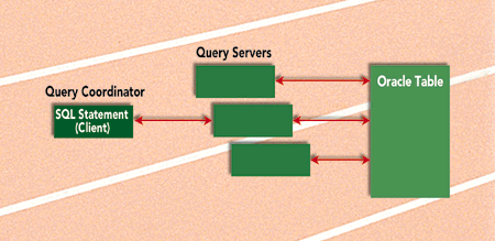
TABLE 1 | ||
|---|---|---|
| - | Nonparallel operation | Parallel operation |
| Elapsed Time | 2 minutes, 50 seconds | 1 minute, 5 seconds |
TABLE 2 | ||
|---|---|---|
| - | Nonparallel operation | Parallel operation |
| Elapsed Time | 7 minutes, 02 seconds | 5 seconds |
TABLE 3 | ||
|---|---|---|
| - | Table Scan | Bitmap Index |
| CPU Time (seconds) | 43.12 | 0.01 |
| Logical Blocks Read | 29282 | 3 |
| Physical Blocks Read | 28778 | 0 |
| Elapsed Tim (seconds) | 1 minute, 35 seconds | 0.07 |
TABLE 4 | ||||
|---|---|---|---|---|
| - | Rule | Cost First | Cost All | Hints |
| Elapsed Time (seconds) | 38.44 | 168.83 | 174.34 | 39.19 |
| CPU Time (seconds) | 14.18 | 150.10 | 154.81 | 30.40 |
| Logical Blocks Read | 29292 | 2870924 | 2870924 | 12826 |
| Physical Blocks Read | 6411 | 10440 | 10459 | 68 |
| Logical Writes | 0 | 0 | 0 | 1082 |
| Recursive Calls | 0 | 0 | 0 | 4588 |
| Database Calls | 3 | 3 | 3 | 24 |